
In control theory, the PID (Proportional–Integral–Derivative) algorithm is often considered the holy grail of control. PID is one of the most successful control algorithms due to its flexibility and simplicity, and it’s relatively easy to implement. In fact, the PID control algorithm has proven robust and flexible enough to yield excellent results in a wide variety of applications, which is a main reason for its continued widespread use over the decades.
The PID algorithm’s flexibility and effectiveness have led to its adoption in countless systems across different domains. Some examples include:
These are just a few examples — PID controllers are employed anywhere we need to automatically maintain a variable at a set value with minimal error. From simple home appliances to critical aerospace systems, PID control provides a reliable way to regulate behavior.
To better understand how the PID algorithm works, let’s consider a simple real-world use case: controlling a robot’s wheel motor to achieve a specific speed.
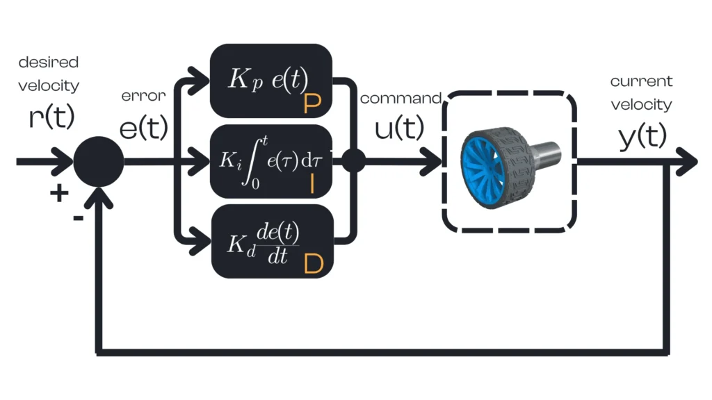
Suppose we want the motor to rotate at a desired speed of 1 radian per second. This target speed is the desired value (also called the setpoint, denoted as \(r(t)\). We can measure the motor’s current speed using an encoder, giving us \(y(t)\) as the feedback output of the system. We then compare the current speed to the setpoint to compute the error \(e(t)\), defined as the difference between the desired and current speed: $$e(t) = r(t) – y(t)$$
The controller’s job is to use this error to generate a command \(u(t)\) (for an electric motor, this command could be a voltage or power level) to drive the error toward zero. In other words, the PID controller will take \(e(t)\) as input and output a control signal \(u(t)\) that minimizes this error, making the motor reach the desired speed as quickly as possible.

Let’s walk through an example scenario step by step:
Because the error is large, the PID controller responds with a large command. For instance, if the motor’s command range is 0 to 255 (where 255 is full power), the controller might output 255 to give maximum thrust. This strong action causes the motor to accelerate quickly.
Throughout this process, the PID controller runs its loop repeatedly (many times per second), each time recalculating the error and adjusting the command. Notice that once the setpoint is reached, the controller doesn’t turn off — it continues working to hold the motor at \(1 rad/s\).
If any disturbance occurs (for example, if the robot starts going uphill or we add a load on the wheel), the error will no longer be zero. The PID loop will then respond by increasing the motor command (drawing more current) to compensate and keep the speed constant.
This closed-loop behavior is what makes PID so powerful: the controller automatically corrects for changes and uncertainties to minimize the error at all times.
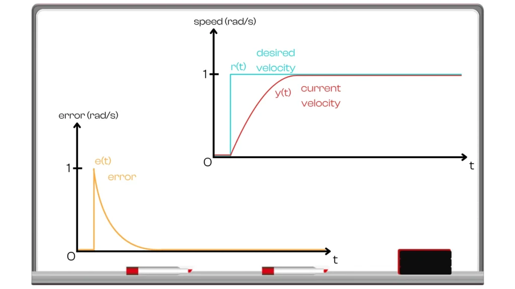
If we visualize the behavior of this PID-controlled motor, we would see the desired speed (setpoint) as a horizontal line at \(1 rad/s\) and the motor’s speed \(y(t)\) gradually rising to meet it. In a well-tuned system, the speed curve will approach the target smoothly without exceeding it (no overshoot). The control input \(u(t)\) starts at a maximum value to kick-start the motion, then steps down as the error decreases, leveling off once the target speed is achieved.
Meanwhile, the error \(e(t)\) begins at \(1 rad/s\) (when the motor is stopped) and steadily declines to 0 as the motor reaches \(1 rad/s\). This example illustrates the essence of PID control: at each moment, the controller computes a command that strives to reduce the error. Over time, the output converges to the setpoint due to the controller’s corrective actions.
In summary, the PID controller generates a control command that continuously pushes the system toward the desired value. By responding strongly when the error is large and backing off as the error shrinks, the PID algorithm drives the error to zero in a reasonable time and then maintains the target with minimal deviation.
So far, we treated the PID controller as a black box that takes an error and outputs a command. Now let’s open that box and see what’s inside. The name PID comes from the three mathematical components at the core of its operation: Proportional, Integral, and Derivative. Each component handles a different aspect of error correction:
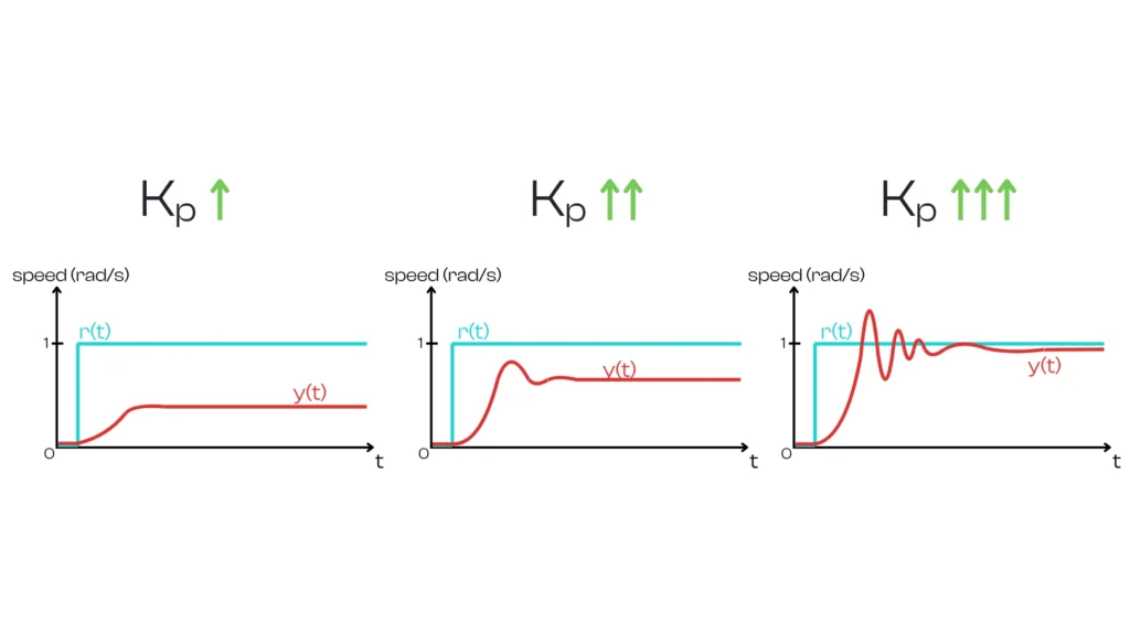
The proportional component generates an output that is proportional to the current error. It essentially looks at how far off the setpoint we are right now. The proportional term output is computed as $$P_\text{out} = K_p \cdot e(t)$$ where \(K_p\) is the proportional gain (a constant) and \(e(t)\) is the instantaneous error. If the error is large, \(P_\text{out}\) will be large; if the error is small, \(P_\text{out}\) will be small. This term’s job is to immediately correct the current error by commanding the actuator in the direction that reduces \(e(t)\). Intuitively, the P term is a straight-line response: for example, if you’re driving and you’re 5 mph below the desired speed, a proportional controller might press the accelerator a certain amount; if you’re 10 mph slow (double the error), it will press twice as much.
However, proportional control on its own has a limitation: it typically cannot drive the error all the way to zero, especially in the presence of external forces or friction. The system tends to stabilize when the proportional output balances out those opposing forces, which often leaves a steady-state error (offset). In our motor example, using only a P term might make the motor stabilize slightly below \(1 rad/s\), because some error is needed to produce enough output to counteract friction. Increasing \(K_p\) reduces this residual error, but one cannot increase \(K_p\) arbitrarily high without consequences (as we’ll discuss in tuning).
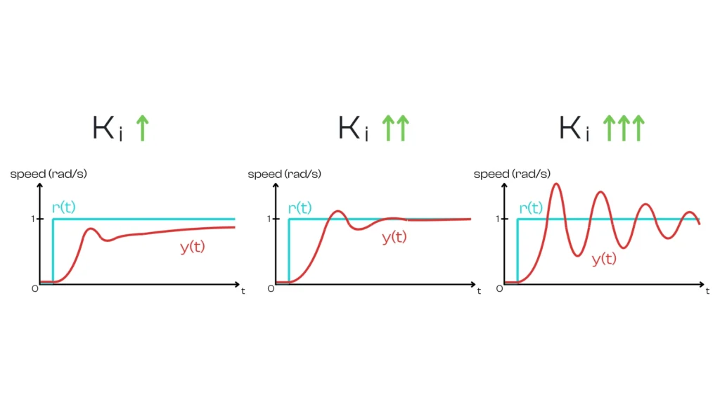
The integral component produces an output proportional to the accumulated error over time. It looks at how long and how far we’ve been off in the past. Mathematically, it integrates the error: $$I_\text{out} = K_i \int e(t),dt$& (the integral of error from the start up to the current time), and \(K_i\) is the integral gain. In practice, the integral term continuously sums up errors: even a small persistent error will accumulate over time into a large integral value.
The role of the I term is to eliminate long-standing, steady errors. It slowly increases the controller output as long as there is any error, and it won’t rest until the error has been driven to zero. Going back to the driving analogy, if your car remains 2 mph below the set speed for a while, the integral term will keep increasing the throttle over that duration, effectively saying “we’ve been off by 2 mph for too long, let’s push a bit more until that error is gone.” Thanks to the integral action, a well-tuned PID controller can remove the steady-state offset that a pure P controller leaves. Once the error is zero (on target), the integral term will stop growing. In fact, if the error becomes positive (meaning you’ve gone above the setpoint), the integral term can start to cancel out (it will decrease, because the error has flipped sign).
One must be careful with the integral term: since it reacts to accumulated past errors, it can make the system slower to respond to changes (it’s a delayed effect), and too much integral action can lead to overshoot. If the integral term has built up a large correction while chasing an error, that momentum can cause the system to overshoot the target and then have to swing back.
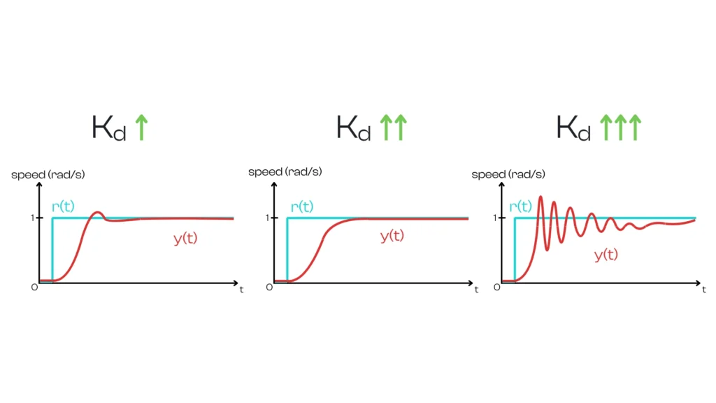
The derivative component’s output is proportional to the rate of change of the error. In essence, it looks at how the error is changing (how it might behave in the future if the trend continues). It is calculated as $$D_\text{out} = K_d \frac{d e(t)}{d t}$$, with \(K_d\) the derivative gain. The derivative term acts like a predictor: it responds to the speed of error change. If the error is decreasing rapidly, the D term will produce a significant output in the opposite direction, effectively applying the brakes to the controller’s action. If the error isn’t changing much or is changing slowly, the D output will be small.
The main purpose of the D term is to dampen the system and reduce overshoot. It anticipates where the error is heading and counteracts fast changes. Imagine driving and approaching the desired speed: if you’re closing in quickly, the derivative term will ease off the accelerator preemptively to avoid overshooting the speed. In a PID-controlled motor, as the speed approaches the setpoint, the D term counters the P term’s push, helping prevent the speed from overshooting and oscillating around the target. A properly tuned derivative term improves stability and settling time. However, the D term is sensitive to noise in measurements (a noisy speed signal can cause large, erratic D outputs), which is why in practice \(K_d\) is often kept relatively small or even zero in many systems.
In other words, the P component addresses the present error, the I component addresses the accumulation of past errors, and the D component attempts to predict future errors based on their current rate of change. By combining these three contributions, a PID controller reacts to what is happening now, what has happened before, and what is likely to happen next. This blend allows it to correct errors efficiently and robustly.
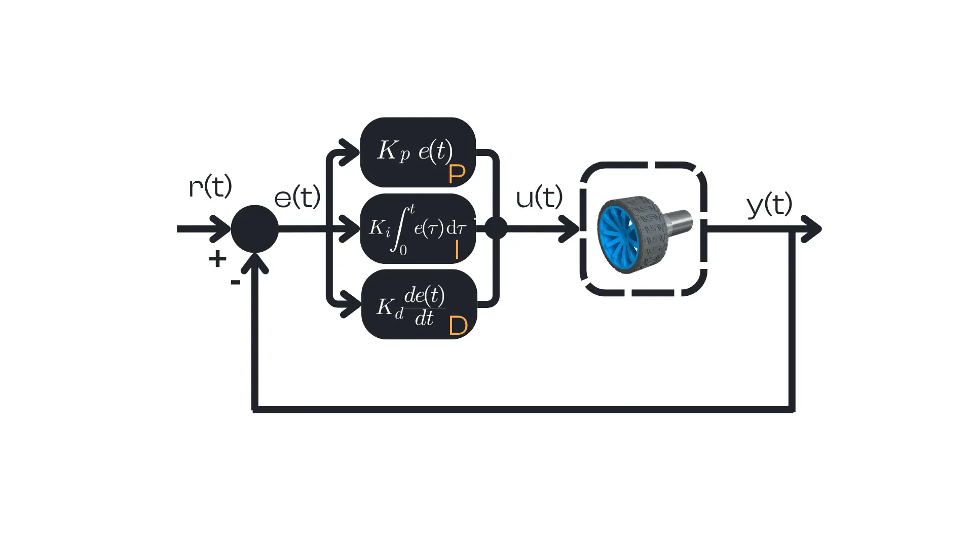
Mathematically, a PID controller in a feedback loop can be expressed with a simple equation. At any time \(t\), given the system’s desired input \(r(t)\) and its measured output \(y(t)\), we define the error as: $$e(t) = r(t) – y(t)$$
The controller computes a control signal (command) \(u(t)\) as the sum of a Proportional term, an Integral term, and a Derivative term:
$$u(t) = K_p \cdot e(t) + K_i \int_0^t e(\tau) \, d\tau + K_d \cdot \frac{d e(t)}{d t}$$
In this formula, \(K_p\), \(K_i\), and \(K_d\) are constants known as the PID gains (proportional gain, integral gain, and derivative gain, respectively). These gains determine the weight or influence of each of the P, I, D components on the controller’s output.
The controller output \(u(t)\) is then applied to the system (for example, as a voltage to the motor) to drive the output \(y(t)\) toward the setpoint \(r(t)\). This equation is the one we will implement in code for our robot’s controller: at each time step, our program will calculate the error and then use this formula to compute the new command to send to the motors.
Notice that the PID formula depends only on the error \(e(t)\) (and its history and rate of change) and on the chosen gains \(K_p\), \(K_i\), \(K_d\). It does not explicitly depend on the time \(t\) itself or any knowledge of the internal dynamics of the system – PID is a generic closed-loop controller. The art of using PID effectively lies in choosing appropriate values for these three gains so that the closed-loop system behaves as desired. This choice is what we call PID tuning.
Assemble your robot and get started to learn Robotics!