Integrating a 2D LiDAR into Your ROS 2 Robot Model

One of the key elements that enables a mobile robot to navigate autonomously is its ability to perceive the surrounding environment.
Among the most widespread and reliable sensors used in robotics is the 2D LiDAR (Light Detection and Ranging).
This device has revolutionized mobile robotics thanks to its accuracy and the ease with which it can be integrated into ROS 2 systems.

In this article, we will analyze how a LiDAR works, what information it provides to the robot, and how to add and simulate it in ROS 2 and Gazebo.

🤔 How a 2D LiDAR Works

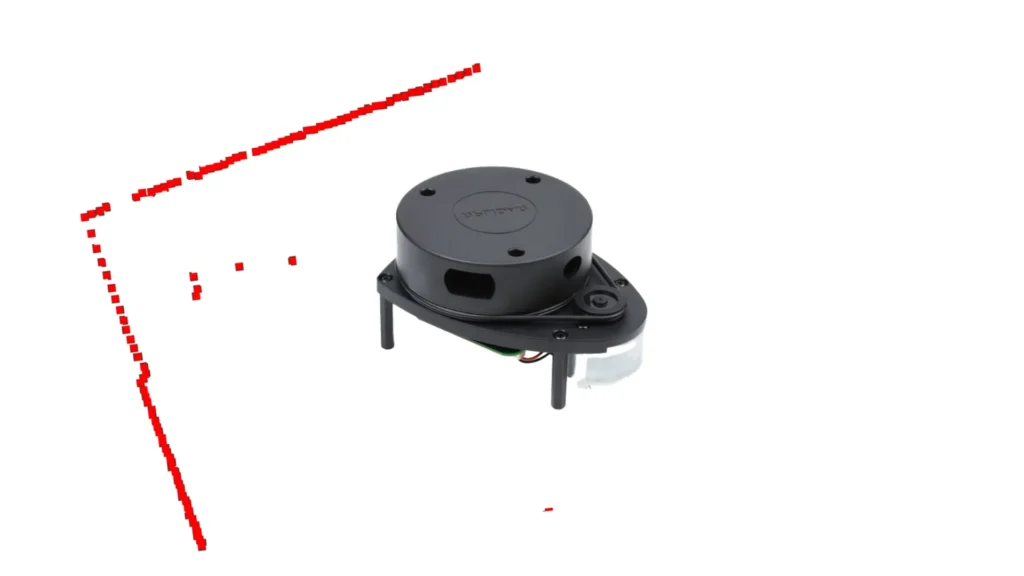
A 2D LiDAR operates by emitting laser beams and measuring the time it takes for the reflected light to return after hitting an object. From this measurement, the sensor computes the distance to obstacles in multiple directions, producing a polar map of the environment.

When repeated hundreds of times per second, these measurements create a two-dimensional point cloud representing the outlines of walls, furniture, and any detected object.

LiDARs provide high precision, often down to a few centimeters, and are capable of scanning up to 360° depending on the model. However, they only capture data on a plane (2D) and can be less effective in outdoor environments with direct sunlight.

In ROS 2, LiDAR data is published on the /scan topic as messages of type sensor_msgs/LaserScan.

📄 Adding a LiDAR to the Robot Model

To integrate a LiDAR sensor into the robot’s model, we need to extend the URDF (Unified Robot Description Format) by defining a new link that represents the sensor and a joint that attaches it to the robot’s base.

The link describes both the visual appearance of the LiDAR (using its mesh file) and its physical properties, such as collision geometry and inertial parameters.

The joint, in turn, establishes how this new link is positioned and connected to the main structure of the robot.

Below is the complete URDF snippet that defines the LiDAR link and its fixed joint connection to the base:

				
					<link name="lidar_link">
  <visual>
    <geometry>
      <mesh filename="package://arduinobot_description/meshes/hokuyo.dae"/>
    </geometry>
  </visual>
  <collision>
    <geometry>
      <cylinder radius="0.05" length="0.05"/>
    </geometry>
  </collision>
  <inertial>
    <mass value="0.1"/>
    <origin xyz="0 0 0" rpy="0 0 0"/>
    <inertia ixx="0.001" iyy="0.001" izz="0.001"
             ixy="0.0" ixz="0.0" iyz="0.0"/>
  </inertial>
</link>

<joint name="lidar_joint" type="fixed">
  <parent link="base_link"/>
  <child link="lidar_link"/>
  <origin xyz="0 0 0.2" rpy="0 0 0"/>
</joint>


🧠 Let’s break down the code

Defining the LiDAR link
				
					<link name="lidar_link">


This line defines a new link named lidar_link, representing the physical body of the sensor inside the robot model.

Visual representation
				
					<visual>
  <geometry>
    <mesh filename="package://arduinobot_description/meshes/hokuyo.dae"/>
  </geometry>
</visual>


The <visual> block specifies the graphical appearance of the sensor, loading a 3D mesh of the Hokuyo LiDAR. This model is used in visualization tools like RViz and Gazebo but does not affect physics.

Collision geometry
				
					<collision>
  <geometry>
    <cylinder radius="0.05" length="0.05"/>
  </geometry>
</collision>


Here we define the simplified collision geometry. Instead of using the complex mesh, a cylinder with 5 cm radius and length is used. This reduces computational load while still approximating the sensor’s shape.

Inertial properties
				
					<inertial>
  <mass value="0.1"/>
  <origin xyz="0 0 0" rpy="0 0 0"/>
  <inertia ixx="0.001" iyy="0.001" izz="0.001"
           ixy="0.0" ixz="0.0" iyz="0.0"/>
</inertial>


The <inertial> block assigns physical properties to the sensor. A mass of 0.1 kg is realistic for a small LiDAR. The origin is aligned with the geometry center, and the inertia matrix defines how the object responds to forces and rotations. Simplified values ensure stable simulation.

Fixed joint connection
				
					<joint name="lidar_joint" type="fixed">
  <parent link="base_link"/>
  <child link="lidar_link"/>
  <origin xyz="0 0 0.2" rpy="0 0 0"/>
</joint>


This section introduces a fixed joint connecting the LiDAR to the robot’s base_link. The <origin> sets the position: the sensor is placed 20 cm above the base without any rotation.

At this point, the LiDAR is fully integrated into the robot’s URDF model.

📊 Simulating the LiDAR in Gazebo

To replicate the behavior of the LiDAR in simulation and obtain data streams within ROS 2, we need to configure a dedicated Gazebo plugin. This plugin generates laser scan data based on the parameters we define, such as update rate, measurement range, angular resolution, and noise model.

The configuration below specifies the ROS topic on which the simulated LiDAR publishes, the reference frame of the sensor, and the physical characteristics of the laser beam, including horizontal scanning limits and the number of samples per scan. By tuning these parameters, we can achieve a realistic simulation that closely matches the performance of the actual hardware.

Here is the full plugin configuration:

				
					<gazebo>
  <plugin name="gazebo_ros_laser" filename="libgazebo_ros_laser.so">
    <ros>
      <namespace>/</namespace>
      <argument>~/scan:=/scan</argument>
    </ros>
    <update_rate>30</update_rate>
    <topicName>/scan</topicName>
    <frameName>lidar_link</frameName>
    <range>
      <min>0.12</min>
      <max>3.5</max>
      <resolution>0.01</resolution>
    </range>
    <ray>
      <scan>
        <horizontal>
          <samples>720</samples>
          <resolution>1</resolution>
          <min_angle>-1.5708</min_angle>
          <max_angle>1.5708</max_angle>
        </horizontal>
      </scan>
      <noise>
        <type>gaussian</type>
        <mean>0.0</mean>
        <stddev>0.01</stddev>
      </noise>
    </ray>
  </plugin>
</gazebo>


🧠 Let’s break down the code

Opening the Gazebo section
				
					<gazebo>


Opens the section with Gazebo-specific tags inside the URDF/Xacro.

Loading the LiDAR plugin
				
					  <plugin name="gazebo_ros_laser" filename="libgazebo_ros_laser.so">


Loads the ROS-Gazebo plugin for simulating a LiDAR sensor.

ROS integration setup
				
					    <ros>
      <namespace>/</namespace>
      <argument>~/scan:=/scan</argument>
    </ros>


Configures integration with ROS 2, publishing the scan on the /scan topic.

Update rate
				
					    <update_rate>30</update_rate>


Sets the update rate to 30 Hz, meaning thirty scans per second.

Topic configuration
				
					    <topicName>/scan</topicName>


Specifies the name of the published topic, ensuring compatibility with navigation stacks.

Reference frame
				
					    <frameName>lidar_link</frameName>


Associates the scans with the lidar_link frame defined in the URDF.

Sensor range
				
					    <range>
      <min>0.12</min>
      <max>3.5</max>
      <resolution>0.01</resolution>
    </range>


Defines the sensor’s range: minimum 12 cm, maximum 3.5 m, with 1 cm resolution.

Scan geometry
				
					    <ray>
      <scan>
        <horizontal>
          <samples>720</samples>
          <resolution>1</resolution>
          <min_angle>-1.5708</min_angle>
          <max_angle>1.5708</max_angle>
        </horizontal>
      </scan>


Describes the scan geometry: 720 beams across 180° (from -1.5708 to +1.5708 radians), providing an angular resolution of ~0.25°.

Noise model
				
					      <noise>
        <type>gaussian</type>
        <mean>0.0</mean>
        <stddev>0.01</stddev>
      </noise>


Adds Gaussian noise with zero mean and 1 cm standard deviation to simulate real-world imperfections.

Closing the plugin definition
				
					  </plugin>
</gazebo>


Closes the plugin definition. Once loaded in Gazebo, the sensor publishes sensor_msgs/LaserScan messages at 30 Hz.

🚀 Testing the Simulation

After updating the URDF and plugin configuration, you can launch the simulation with:

				
					ros2 launch arduinobot_gazebo simulated_robot.launch.py


Then, in a new terminal, check the data being published:

				
					ros2 topic echo /scan


You should see a stream of range values corresponding to the distances measured by the LiDAR’s beams.

In this article, we explored how a 2D LiDAR works, how to integrate it into the robot’s URDF model, and how to simulate it in Gazebo to generate realistic scan data. This type of sensor is one of the most powerful and versatile tools for autonomous navigation, forming the foundation for mapping, localization, and obstacle avoidance.


Want to learn more?

Discover how to design, build, and use maps in real robotic systems in the "Self Driving and ROS 2 - Learn by doing! Map & Localization" course
DISCOUNT
en_US