
When we move from simple robot experiments to real-world navigation, the environment is no longer an abstract concept. A robot needs to understand where it can move, where it cannot, and how to plan paths that are not only valid but also safe and efficient. This is where costmaps come into play in ROS 2 Navigation (Nav2).
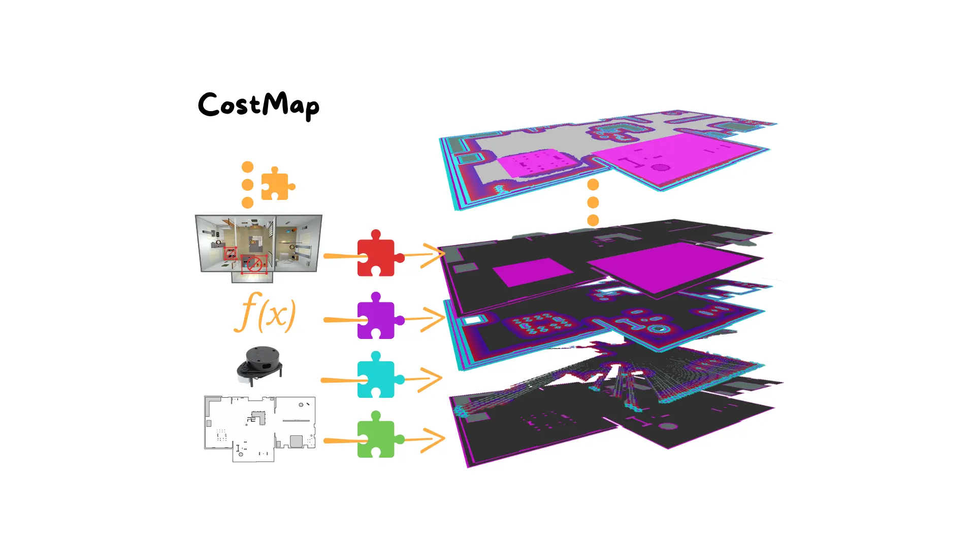
A costmap is essentially a grid-based representation of the environment, where each cell carries a “cost” that indicates how desirable or undesirable it is for the robot to step into it. Free space has low cost, obstacles have high cost, and unsafe zones around obstacles are inflated to discourage risky paths. By combining different layers of information, costmaps provide a comprehensive, real-time view of the robot’s surroundings.
In this article, we will dive into the theory behind costmaps and then build a full Nav2 costmap configuration using three essential layers: the static layer, the obstacle layer, and the inflation layer. At the end, you will have a working configuration file, fully explained line by line, that you can plug into your robot’s navigation system.
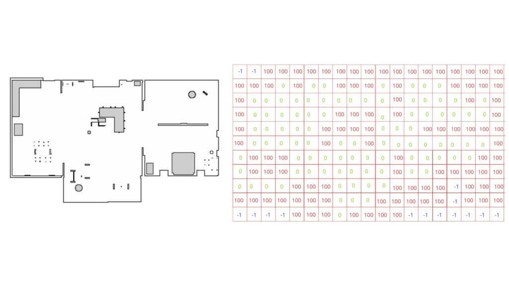
At its core, a costmap is a 2D grid laid over the robot’s environment. Each cell in this grid contains an integer value:
0 represents free space
100 represents an obstacle
values in between represent inflated or uncertain zones
This grid allows Nav2 to perform collision checking and path planning efficiently. Rather than reasoning about the entire geometry of the robot and the environment, the system just checks the costs of cells and looks for low-cost paths.
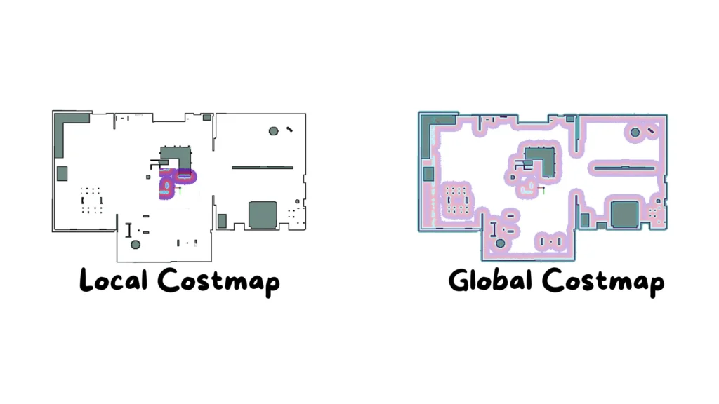
In Nav2, we typically define two separate costmaps. The global costmap provides a large-scale, static view of the environment, usually aligned with the map, and is used for long-term path planning. The local costmap instead provides a smaller, robot-centered view, updated at a higher frequency, and accounts for dynamic obstacles, enabling local replanning and obstacle avoidance.
By combining the two, the robot can plan safe long-distance routes while also reacting in real-time to sudden changes in the environment.
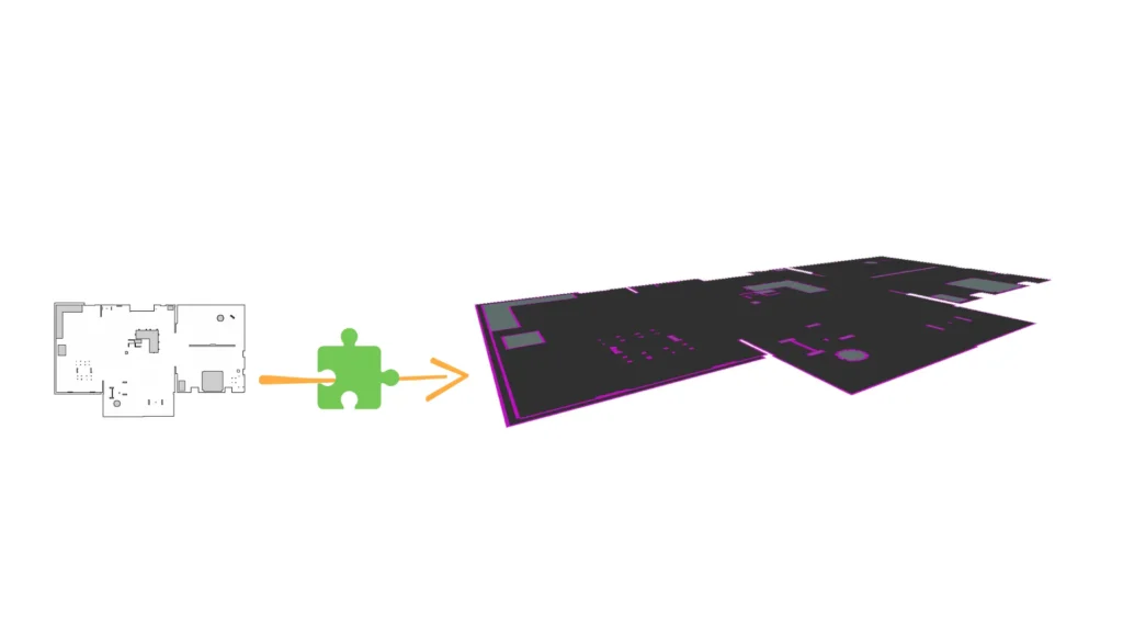
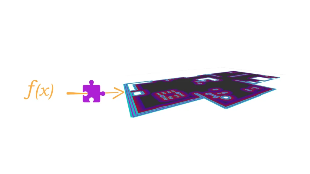
The static layer imports information from a pre-built occupancy grid map, usually the one generated by SLAM or mapping. By subscribing to /map, it guarantees that the costmap reflects static structures like walls and corridors.
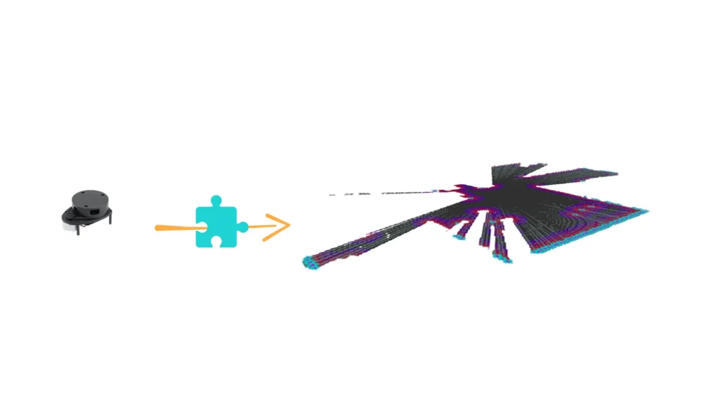
The obstacle layer integrates sensor data from LiDAR or depth cameras to detect obstacles in real-time. It listens to topics like /scan and constantly updates the costmap, ensuring dynamic objects are considered.
The inflation layer expands the occupied areas detected in the costmap, effectively creating a buffer zone around obstacles. This prevents the robot from planning paths that pass dangerously close to walls or objects. Parameters like inflation_radius and cost_scaling_factor determine how wide and steep this buffer is.
We are now ready to implement a working costmap in ROS 2. Costmaps are configured using YAML parameter files. Let’s create a file called costmap_params.yaml inside the config folder of our navigation package.
					# costmap_params.yaml
nav2_costmap_2d:
  global_costmap:
    ros__parameters:
      global_frame: map
      robot_base_frame: base_link
      update_frequency: 10.0
      publish_frequency: 10.0
      resolution: 0.05
      width: 10
      height: 10
      origin_x: 0.0
      origin_y: 0.0
      plugins: ["static_layer", "obstacle_layer", "inflation_layer"]

      static_layer:
        plugin: "nav2_costmap_2d::StaticLayer"
        map_subscribe_transient_local: true

      obstacle_layer:
        plugin: "nav2_costmap_2d::ObstacleLayer"
        observation_sources: laser_scan_sensor
        laser_scan_sensor:
          topic: /scan
          clearing: true
          marking: true
          data_type: "LaserScan"
          inf_is_valid: true

      inflation_layer:
        plugin: "nav2_costmap_2d::InflationLayer"
        inflation_radius: 0.55
        cost_scaling_factor: 10.0
We now break down the file, section by section, and explain what each parameter does.
					nav2_costmap_2d:
  global_costmap:
    ros__parameters:
This opens the costmap configuration inside the nav2_params file. The section ros__parameters will contain all the parameters that define how the costmap works.
					      use_sim_time: true
      global_frame: map
      robot_base_frame: base_link
Here we enable simulation time (use_sim_time: true) so the costmap synchronizes with Gazebo or another simulator. The global_frame is set to map so all obstacle positions are relative to the global map. The robot_base_frame indicates the robot’s main reference frame, usually base_link.
					      update_frequency: 5.0
      publish_frequency: 2.0
      resolution: 0.05
The update frequency determines how often the costmap integrates new sensor data (in Hz), while the publish frequency sets how often the costmap is broadcast to other nodes. The resolution defines the grid cell size in meters — in this case, each cell is 5 cm.
					      width: 10.0
      height: 10.0
      origin_x: -5.0
      origin_y: -5.0
These parameters configure the costmap’s size in meters and where it is centered. A width and height of 10 meters with origin at -5,-5 places the costmap symmetrically around the robot.
					      plugins:
        - {name: static_layer, type: "nav2_costmap_2d::StaticLayer"}
      static_layer:
        map_subscribe_transient_local: true
The static layer plugin loads the environment map. The option map_subscribe_transient_local ensures the costmap always receives the map even if it was published before the costmap started.
					        - {name: obstacle_layer, type: "nav2_costmap_2d::ObstacleLayer"}
      obstacle_layer:
        observation_sources: scan
This section enables the obstacle layer. It subscribes to one or more sensor topics, in this case just scan, which is usually the LiDAR data.
					        scan:
          topic: /scan
          max_obstacle_height: 2.0
          clearing: true
          marking: true
The obstacle data comes from /scan. Any obstacle taller than 2 meters is ignored. Marking adds detected obstacles into the costmap, while clearing removes them when the sensor no longer detects them.
					        - {name: inflation_layer, type: "nav2_costmap_2d::InflationLayer"}
      inflation_layer:
        inflation_radius: 0.55
        cost_scaling_factor: 10.0
The inflation layer creates a safety buffer around obstacles. The inflation_radius determines how far costs spread, and the cost_scaling_factor adjusts how quickly the costs decay with distance from obstacles.
With the configuration in place, we can build and run the navigation stack.
					cd ~/arduinobot_ws
colcon build
source install/setup.bash
ros2 launch nav2_bringup bringup_launch.py params_file:=/path/to/costmap_params.yaml
Opening RViz will show the costmap overlayed on the map. Obstacles will appear as blocked areas, and inflated zones will surround them as gray gradients, making it clear where the robot can move safely.
Costmaps are a fundamental part of robot navigation in ROS 2. They combine static knowledge from maps, dynamic perception from sensors, and safety margins from inflation, resulting in a layered representation of the environment. In this article, we explored the theory behind costmaps, then implemented a complete configuration with static, obstacle, and inflation layers, and finally explained each section of the code in detail.
With this setup, your robot can plan paths that are not only feasible but also safe, handling both static maps and dynamic environments.
Assemble your robot and get started to learn Robotics!