
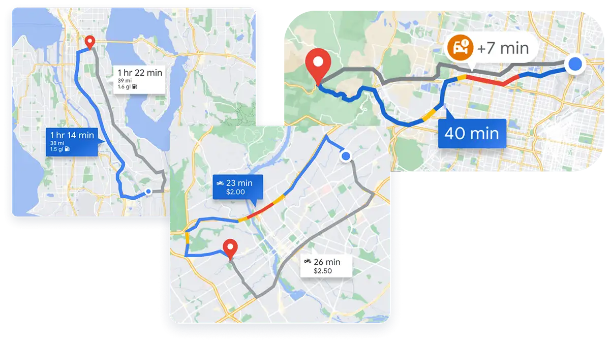
Ever stared at Google Maps, marveling at how it instantly whips up the best route through a chaotic city, rerouting on the fly for traffic jams you didn’t even know existed? We take it for granted. But this “magic” is the result of decades of work on problems that, at their core, are about finding the most efficient way from A to B.
Now, translate that to robotics. Your autonomous mobile robot isn’t (yet) navigating the streets of Rome, but the fundamental challenge is identical. It needs:
This isn’t just about getting from A to B. It’s about doing it smartly. The fastest way? The shortest? The safest? The one that uses the least energy? These are the questions that separate a toy from a tool.
It’s crucial to understand that planning is only half the battle. A Planner is your high-level strategist. It looks at the map, the start, the goal, and charts a course. Think of it as deciding to take the M5 motorway, then exit 15.
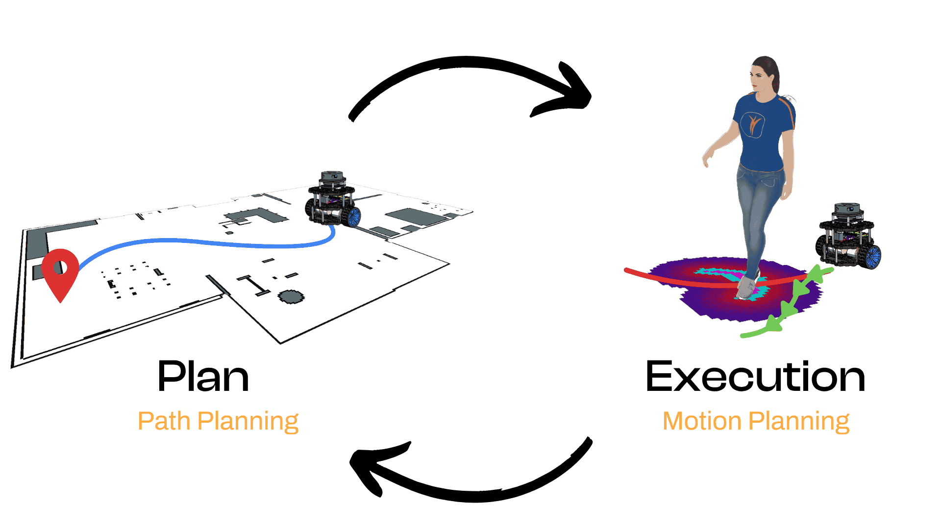
An Executor (often called a Motion Planner or Local Planner) is your tactical officer in the field. It takes the high-level plan and deals with the messy reality: staying in the lane, avoiding that pedestrian who just stepped out, yielding to other vehicles. It’s the system that slams the brakes or nudges the robot slightly to avoid an unexpected obstacle.
These two systems are in constant dialogue. The executor feeds new information about the environment (e.g., an unexpected blockage) back to the planner, which might then recalculate a better high-level route. This feedback loop is critical for robust autonomy.
In this post, we’re dissecting the Planner, specifically how we can use algorithms like Dijkstra’s to find that optimal high-level path.
To make a computer plan a path, we can’t just throw a raw image of the environment at it. We need to abstract and simplify.
2. Continuous to Discrete: The Power of Grids and Graphs: The C-Space is still continuous. Computers prefer discrete data. The most common way to handle this for grid maps (like the OccupancyGrid in ROS) is Cell Decomposition. We overlay a grid onto our C-Space. Each cell is either free or occupied. Now, we can represent this grid as a graph. Each free cell becomes a node (or vertex) in our graph. If two free cells are adjacent (up, down, left, right), we draw an edge connecting their corresponding nodes. Each edge can have a cost. For simple grid navigation, the cost to move from one cell to an adjacent one is often 1. But it could represent actual distance, traversal time, energy cost, or any other metric you want to optimize.
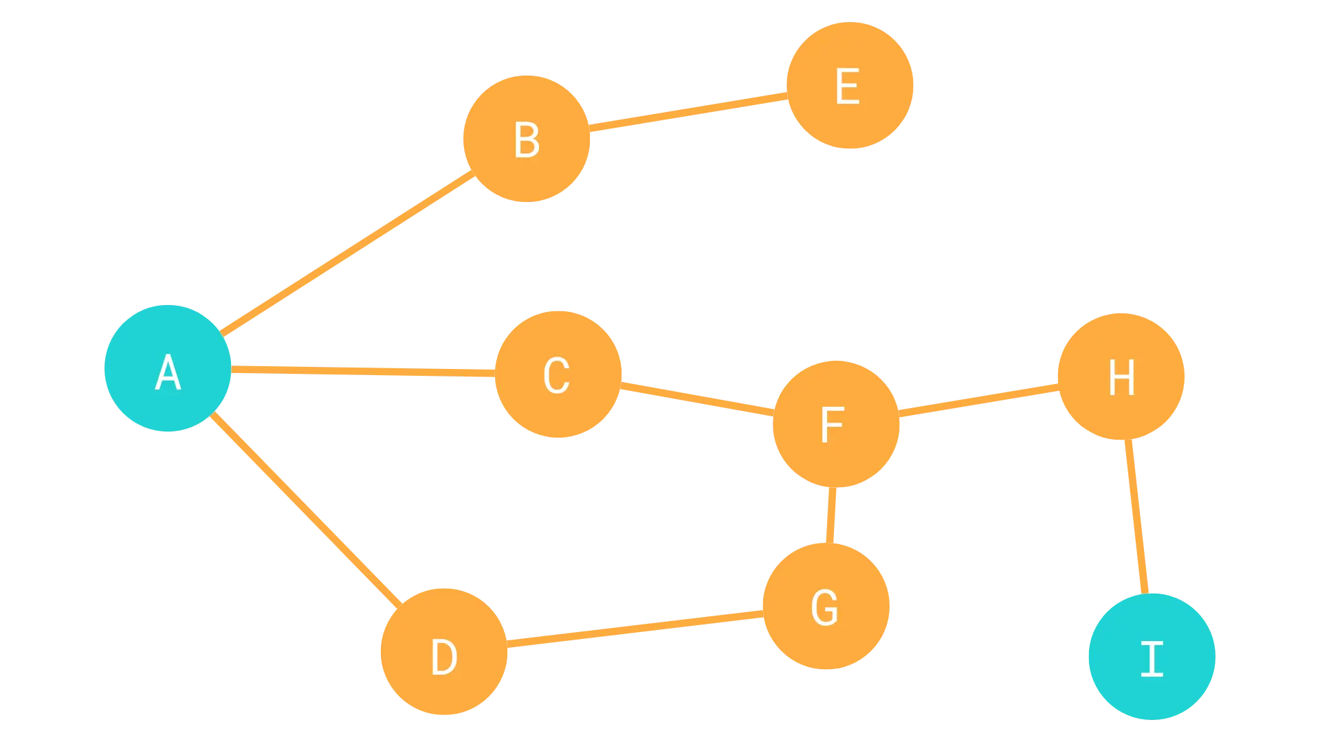
Now, the path planning problem is transformed: Find the sequence of edges in this graph that connects the start node to the goal node with the minimum total cost.
Dijkstra’s algorithm is a cornerstone for finding the shortest path in a weighted graph where edge weights are non-negative (which they usually are for distance or basic cost). It systematically explores the graph, always expanding from the “closest” node it hasn’t fully processed yet.
Here’s the core idea:
While the priority queue is not empty and the goal hasn’t been reached: a. Extract the node with the smallest cost (let’s call it current_node) from the priority queue. b. Mark current_node as visited. c. If current_node is the goal node, we’re done! Reconstruct the path by backtracking using stored predecessor information. d. For each neighbor of current_node that hasn’t been visited: i. Calculate the cost to reach this neighbor through current_node (cost to current_node + cost of edge from current_node to neighbor). ii. If this new cost is less than any previously known cost to reach the neighbor, update the neighbor’s cost and record current_node as its predecessor. Add/update the neighbor in the priority queue.
This methodical exploration guarantees that when you reach the goal node, you’ve found the shortest path to it.
Let’s look at how this translates into a ROS 2 Python node. The code you’re working with implements Dijkstra for an OccupancyGrid.
					#!/usr/bin/env python3

import rclpy
from rclpy.node import Node
from nav_msgs.msg import OccupancyGrid, Path
from geometry_msgs.msg import PoseStamped, Pose
from rclpy.qos import QoSProfile, DurabilityPolicy
from tf2_ros import Buffer, TransformListener, LookupException
from queue import PriorityQueue

class GraphNode:
    def __init__(self, x, y, cost=0, prev=None):
        self.x = x
        self.y = y
        self.cost = cost
        self.prev = prev

    def __lt__(self, other):
        return self.cost < other.cost

    def __eq__(self, other):
        return self.x == other.x and self.y == other.y

    def __hash__(self):
        return hash((self.x, self.y))

    def __add__(self, other):
        return GraphNode(self.x + other[0], self.y + other[1])

class DijkstraPlanner(Node):
    def __init__(self):
        super().__init__("dijkstra_node")
        self.tf_buffer = Buffer()
        self.tf_listener = TransformListener(self.tf_buffer, self)

        map_qos = QoSProfile(depth=10)
        map_qos.durability = DurabilityPolicy.TRANSIENT_LOCAL

        self.map_sub = self.create_subscription(
            OccupancyGrid, "/map", self.map_callback, map_qos
        )
        self.pose_sub = self.create_subscription(
            PoseStamped, "/goal_pose", self.goal_callback, 10
        )
        self.path_pub = self.create_publisher(Path, "/dijkstra/path", 10)
        self.map_pub = self.create_publisher(OccupancyGrid, "/dijkstra/visited_map", 10)

        self.map_ = None
        self.visited_map_ = OccupancyGrid()

    def map_callback(self, map_msg: OccupancyGrid):
        self.map_ = map_msg
        self.visited_map_.header.frame_id = map_msg.header.frame_id
        self.visited_map_.info = map_msg.info
        self.visited_map_.data = [-1] * (map_msg.info.height * map_msg.info.width)

    def goal_callback(self, pose: PoseStamped):
        if self.map_ is None:
            self.get_logger().error("No map received!")
            return

        self.visited_map_.data = [-1] * (self.visited_map_.info.height * self.visited_map_.info.width)

        try:
            map_to_base_tf = self.tf_buffer.lookup_transform(
                self.map_.header.frame_id, "base_footprint", rclpy.time.Time()
            )
        except LookupException:
            self.get_logger().error("Could not transform from map to base_footprint")
            return

        map_to_base_pose = Pose()
        map_to_base_pose.position.x = map_to_base_tf.transform.translation.x
        map_to_base_pose.position.y = map_to_base_tf.transform.translation.y
        map_to_base_pose.orientation = map_to_base_tf.transform.rotation

        path = self.plan(map_to_base_pose, pose.pose)
        if path.poses:
            self.get_logger().info("Shortest path found!")
            self.path_pub.publish(path)
        else:
            self.get_logger().warn("No path found to the goal.")

    def plan(self, start: Pose, goal: Pose):
        # Define possible movement directions (4-connectivity)
        explore_directions = [(-1, 0), (1, 0), (0, -1), (0, 1)] # Left, Right, Down, Up

        pending_nodes = PriorityQueue()
        visited_nodes = set() # To keep track of grid cells we've already processed

        start_node = self.world_to_grid(start)
        goal_node_coords = self.world_to_grid(goal) # For checking if goal is reached

        pending_nodes.put(start_node)

        active_node = None # To store the final node if path is found

        while not pending_nodes.empty() and rclpy.ok():
            active_node = pending_nodes.get()

            if active_node == goal_node_coords: # Using __eq__ of GraphNode
                break

            if active_node in visited_nodes: # Already found a shorter path to this node
                continue
            visited_nodes.add(active_node)

            # Visualize explored area
            if self.pose_on_map(active_node): # Check bounds before writing
                 self.visited_map_.data[self.pose_to_cell(active_node)] = 50 # Mark visited

            for dir_x, dir_y in explore_directions:
                new_node_coords: GraphNode = active_node + (dir_x, dir_y) # Create potential new node

                # Check if new_node is valid: within map bounds, not an obstacle, and not visited with a lower cost
                if (self.pose_on_map(new_node_coords) and
                        self.map_.data[self.pose_to_cell(new_node_coords)] == 0 and # 0 means free space
                        new_node_coords not in visited_nodes):

                    new_node_cost = active_node.cost + 1 # Assuming cost of 1 for each step

                    # This is a simplified Dijkstra; for a true version, you'd check if new_node_coords
                    # is already in pending_nodes with a higher cost and update it.
                    # PriorityQueue handles putting it in the right order based on cost.
                    new_node = GraphNode(new_node_coords.x, new_node_coords.y, new_node_cost, active_node)
                    pending_nodes.put(new_node)

            # Publish visited map for visualization periodically (optional, can be slow)
            # self.map_pub.publish(self.visited_map_)


        # Path Reconstruction
        path = Path()
        path.header.frame_id = self.map_.header.frame_id
        path.header.stamp = self.get_clock().now().to_msg() # Add timestamp

        # Check if goal was reached (active_node should be goal_node_coords)
        if active_node and active_node == goal_node_coords:
            current_path_node = active_node
            while current_path_node and rclpy.ok(): # Backtrack from goal to start
                world_pose: Pose = self.grid_to_world(current_path_node)
                pose_stamped = PoseStamped()
                pose_stamped.header.frame_id = self.map_.header.frame_id
                pose_stamped.header.stamp = path.header.stamp # Use same timestamp for all poses
                pose_stamped.pose = world_pose
                path.poses.append(pose_stamped)
                if self.pose_on_map(current_path_node): # Mark path on visited map
                    self.visited_map_.data[self.pose_to_cell(current_path_node)] = 100 # Mark path
                current_path_node = current_path_node.prev
            path.poses.reverse() # Path is reconstructed backwards, so reverse it

        self.map_pub.publish(self.visited_map_) # Publish final visited map with path
        return path

    def pose_on_map(self, node: GraphNode):
        return 0 <= node.x < self.map_.info.width and 0 <= node.y < self.map_.info.height

    def world_to_grid(self, pose: Pose) -> GraphNode:
        grid_x = int((pose.position.x - self.map_.info.origin.position.x) / self.map_.info.resolution)
        grid_y = int((pose.position.y - self.map_.info.origin.position.y) / self.map_.info.resolution)
        return GraphNode(grid_x, grid_y) # Cost and prev are set later

    def grid_to_world(self, node: GraphNode) -> Pose:
        pose = Pose()
        # Center of the cell
        pose.position.x = node.x * self.map_.info.resolution + self.map_.info.origin.position.x + self.map_.info.resolution / 2.0
        pose.position.y = node.y * self.map_.info.resolution + self.map_.info.origin.position.y + self.map_.info.resolution / 2.0
        return pose

    def pose_to_cell(self, node: GraphNode): # Converts (x,y) grid coordinate to 1D array index
        return node.y * self.map_.info.width + node.x


def main(args=None):
    rclpy.init(args=args)
    node = DijkstraPlanner()
    rclpy.spin(node)
    rclpy.shutdown()

if __name__ == '__main__':
    main()
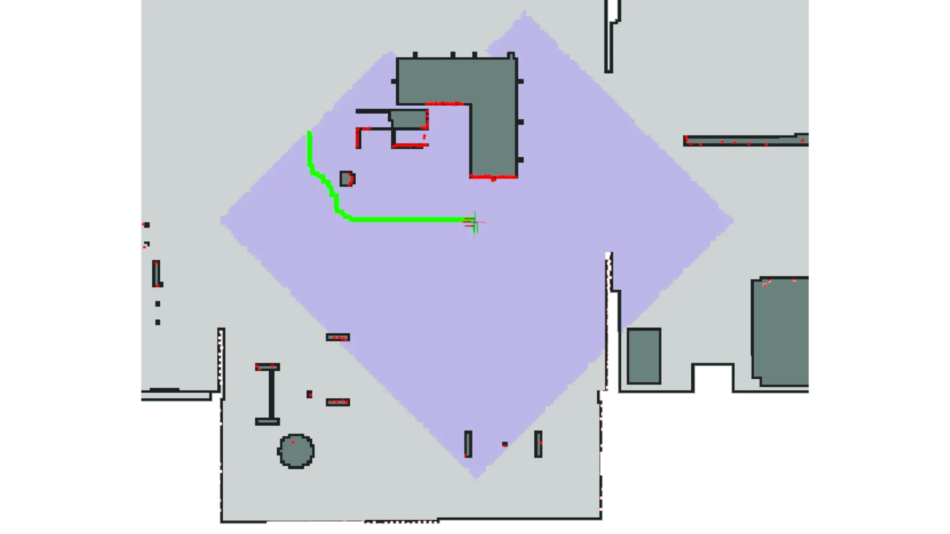
At its heart, the algorithm translates the robot’s map into a grid and then plays a game of finding the shortest path from a start point to a goal.
One of the most clever parts of the algorithm is how it decides where to look next. It doesn’t explore randomly; it expands along a “frontier” of cells, always prioritizing the one with the lowest travel cost from the start. This is managed by the PriorityQueue.
It is a data structure available in the queue Python library:
					from queue import PriorityQueue
...

pending_nodes = PriorityQueue()
The magic that makes this queue “smart” lies in the custom GraphNode class. By defining the __lt__ (less-than) method, we tell the queue how to compare two nodes: the one with the lower cost is considered “smaller.”
					class GraphNode:
      def __init__(self, x, y, cost=0, prev=None):
        self.x = x
        self.y = y
        self.cost = cost
        self.prev = prev

      def __lt__(self, other):
        return self.cost < other.cost

      def __eq__(self, other):
        return self.x == other.x and self.y == other.y

      def __hash__(self):
        return hash((self.x, self.y))

      def __add__(self, other):
        return GraphNode(self.x + other[0], self.y + other[1])
Every time the algorithm discovers a valid new cell to explore, it’s added to this queue. The PriorityQueue automatically handles the sorting, ensuring the next cell to be processed is always the most promising one (i.e., the cheapest to get to).
					# From the plan() function
new_node = GraphNode(new_node_coords.x, new_node_coord.y, new_node_cost, active_node)
pending_nodes.put(new_node)
To be efficient and avoid getting stuck in loops, the algorithm needs a memory of where it’s already been. A Python set is the perfect tool for this job, as it provides a very fast way to check if an item is present.
We initialize the set at the beginning of the planning process:
visited_nodes = set()
Then, inside the main loop, before we do any heavy processing on a node, we first check if we’ve seen it before. If we have, we simply skip it. Because of our PriorityQueue, we know that the first time we visit a node, we have found the shortest path to it.
					# From the plan() function
active_node = pending_nodes.get()
...
if active_node in visited_nodes: # Already found a shorter path here
    continue
visited_nodes.add(active_node) # Mark this node as explored
This simple check is a critical optimization that keeps the search algorithm fast and effective.
This is the engine that drives the search. The while loop systematically executes a simple, repeatable process: pull the best node from the frontier, evaluate its neighbors, and add any valid new ones back to the frontier. This continues until the goal is found.
The loop runs as long as there are still potential cells to explore:
					while not pending_nodes.empty() and rclpy.ok():
    # 1. Select the best node from the frontier
    active_node = pending_nodes.get()

    # 2. If it's the goal, we're done with the search!
    if active_node == goal_node_coords:
        break

    # 3. Otherwise, check all its neighbors
    for dir_x, dir_y in explore_directions:
        # ... code to check if the neighbor is valid ...

        # 4. If valid, create the new node and add it to the frontier
        new_node = GraphNode(...)
        pending_nodes.put(new_node)
Once the loop finds the goal, it needs to build the final path. This is where the prev attribute on our GraphNode comes in. Each time we find a new node, we link it to the node it came from, creating a trail of breadcrumbs. To build the path, we just work our way backward from the goal.
					# Path Reconstruction
current_path_node = active_node # Start at the goal
while current_path_node: # As long as we haven't reached the start
    # Add the current node's position to our path
    path.poses.append(pose_stamped)
    # Move to the previous node in the chain
    current_path_node = current_path_node.prev

# The path is built backward, so we reverse it for the correct order
path.poses.reverse()
And that’s it! By combining a PriorityQueue for intelligent searching, a set for efficient memory, and a simple backtracking method, the algorithm can effectively discover the shortest path in the map.
Time to put all the boring theory into practice and create some cool maps!
Clone the Self-Driving-and-ROS-2-Learn-by-Doing-Plan-Navigation repository on your PC
git clone https://github.com/AntoBrandi/Self-Driving-and-ROS-2-Learn-by-Doing-Plan-Navigation.git
Go to the bumperbot workspace folder in the Section4_Path_Planning folder
cd Self-Driving-and-ROS-2-Learn-by-Doing-Plan-Navigation/Section4_Path_Planning/bumperbot_ws/
Install all the required dependencies using rosdep
rosdep install --from-paths src -y --ignore-src
Once all the dependencies have been installed, build the workspace with
colcon build
In a new window of the terminal, source the bumperbot_ws
. install/setup.bash
Launch the simulation and start planning!
ros2 launch bumperbot_bringup simulated_robot.launch.py world_name:=small_house
Once the simulation is up and running, you can open a new window of the terminal, source the bumperbot_ws also in the new window, and run the dijkstra_planner node.
					. install/setup.bash
ros2 run bumperbot_planning dijkstra_planner.py
In RViz2, add the visualization of the /dijkstra/path and /dijkstra/visited_map topics
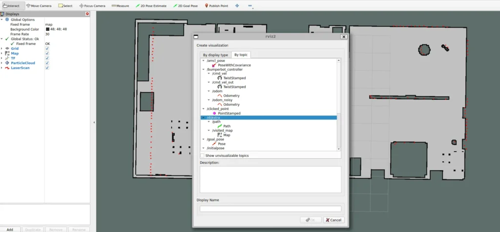
Then, you can finally use the “2D Goal Pose” RViz tool to select a pose in the map and trigger the planner.
Assemble your robot and get started to learn Robotics!